Study of a teaching room
This tutorial concerns the simple study of a teaching room. The geometry is rectangular of size (6m x 10m x 3m). The goal of this tutorial is to:
manipulate face elements
manipulate surface material
manipulate punctual receivers
manipulate omnidirectional sound sources
perfome calculations with the TCR and SPPS codes
display results
Resources for this tutorial are located in the following folder:
<I-Simpa installation folder>\doc\tutorial\tutorial 1
This folder contains several files:
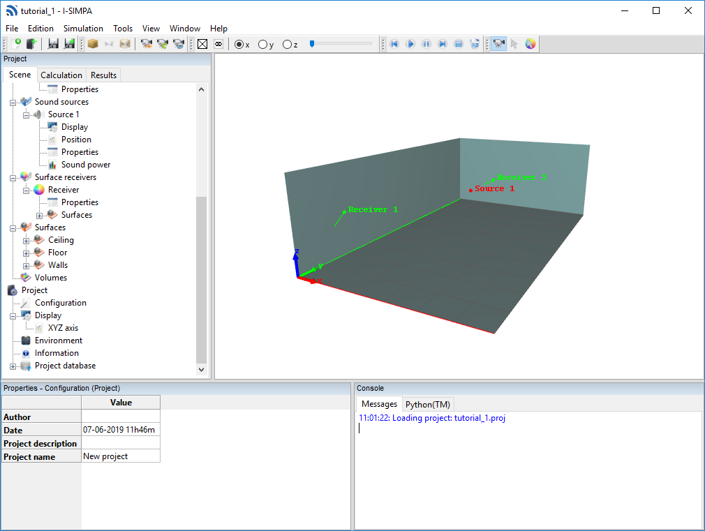
tutorial_1.proj: I-Simpa project of the present tutorial (with TCR and SPPS results)Screenshot_tutorial_1.PNG: I-Simpa screenshot of tutorial 1additional PNG images (screenshots)
Scene creation
Create a new geometry
The first step is to create the geometry. As we consider a simple rectangular geometry with the same material of each mean face, the built-in option for creating a rectangular room can be used.
Note
Remember that for more complicate room shapes of for rectangular room with different materials on a same main face, user will have to create the geometry with a CAD software.
Start I-Simpa
When starting I-Simpa, the default project is the last saved project. To clear I-Simpa, select “New project” in the File menu or click on the “New project” icon on the “File” toolbar to clear I-Simpa
In the menu file, select “New scene”.
Enter the given size of the room (width: 6m, length: 10m and height: 3m), then click on “OK”.
The “Loading 3D scene” windows appears. Leave the default values (you can also deselect all options; this will not change the result) and click on “OK”.
Define surfaces
The second step is to affect one material for each main faces. Here, we will consider 3 surface groups: the “Floor”, the “Walls” and the “Ceiling”.
Select the mode “Face selection” on the toolbar “Selection”
Hold the CTRL key and double-click on the floor in the “3D view”:
this will select all co-planar faces (i.e. both triangular faces of the floor);
the 2 corresponding elements will be underlined in the “Surface” folder of the tree “Data”;
Uses the right click on one of the 2 selected “Surface” elements in the surfaces group in the Scene tree: a contextual menu will appear, and Select “Send to a new face group”
a new surface group, named “group”, is created.
Note
A new group is created with the default name “group”. Group surfaces can have the same name, , since each group is identified with its own internal Id.
Right click on the new corresponding group and Select “Rename” to rename the group with the name “floor” (you can also use the Left click on the group name to change the name)
Astuce
Instead of using the “Face selection” mode, you can create 2 new groups (“Floor” and “Ceiling” for example), select the corresponding surfaces within the “Group” folder and send them to a new face group. You can also directly move the corresponding surfaces to their corresponding surfaces group using the pointer.
Once the surface groups are defined, Left click on a group and select a material in the Material list element in the Properties windows. Repeat the procedure for each surface group, with the following material (for example): Ceiling: “30% absorbing”, Floor: “10% absorbing”, Walls: “20% absorbing”
Define a sound source
Right click on the “Sound sources” root folder in the Data tree of the Scene tab and Select “New source”. A new source is created.
Select the “Position” element and gives the values of the source coordinates (3, 5, 1.8).
Select the “Sound power” element and Choose the “White noise” spectrum in the Spectrum list (it should be the default spectrum).
In the “Global” element of the “Sound power” properties, Defines the value “80” for the “Global” value of the “Lw” tab element. This will define a global sound power of 80 dB.
Define a surface receiver
Right click on the “Surface receiver” root folder in the Data tree of the Scene tab and Select “New scene receiver”. A new surface receiver is created.
In the “Surfaces” root folder, Select the “Floor” group (Left click and Hold) and move it in the “Surfaces” element of the surface receiver. It will define a surface receiver on the room floor.
Define two punctual receivers
Right click on the “Punctual receiver” root folder in the Data tree of the Scene tab and Select “New receiver”. A new punctual receiver is created.
Select the “Position” element and define the coordinates (x,y,z) of the punctual receiver. You can choose (1.,1.,1.8) for example.
Repeat the two fiorst step for the second receiver at location (3.,7.,1.8) for example.
Calculation
TCR code
Select the “Meshing” element in the “Classical theory of reverberation” code.
Enable the “Surface receivers constraint”.
In the “Surface receivers constraint (m²)” element, Define the value “0.1”. This allows to resample the corresponding surfaces for the surface receiver. In the other hand (without defining a surface receiver constraint), only the two initial surface element of the floor will be used as receiver, leading to a very poor definition.
Right click on the “Classical theory of reverberation” and Select “Run calculation” to start the simulation.
SPPS code
1-3. Repeat the same 1-3 steps as for the TCR code.
Right click on the “SPPS” and Select “Run calculation” to start the simulation.
Results
Note
The “Results” tab correspond exactly on the image of the data on the hard disk. You can open the file explorer by a Right click on a result folder and by selecting “Open folder”. You can delete a folder or a file, either using the file explorer or the “Delete” action (Right click on the folder/element in the results folder) within I-Simpa.
Note
For each new simulation, a specific folder in created in the corresponding simulation folder (i.e. SPPS or TCR), with a name that is defined from the starting time and date of the simulation.
Astuce
Most of results are displayed in table. You can select cells in the table, right click on the selection and select “New diagram” to create a graphical display of the results. You can also export data to a csv file by selecting “Save data as…”.
TCR code
Unfold the “Results” folder in the “Classical theory of reverberation” folder.
Unfold the “Punctual receiver” folder, and Double left click on one element (i.e. one of the two receivers that have been created). A new window is displayed, showing the SPL at the receiver for the direct field and the total field (diffuse field + direct field) according to the Sabine and Eyring formulae.
Unfold the “Total field” folder (Sabine or Eyring), Select the surface receiver, Select the frequency band and Right click on the “Sound level” element and Choose “Load animation”, then “Cumulating sound level”. It displays the sound map for the corresponding surface receiver on the 3D view. You can remove the colormap on the 3D view by clicking on the “Dash” icon on the “Simulation” toolbar.
Double left click on the “Main results”. It opens a new display with some general results for the whole room (global reverberation time, SPL of the diffuse sound field and equivalent absorption according to the Sabine and Eyring formulae)
SPPS code
Unfold the “Results” folder in the “SPPS” folder.
Unfold the “Punctual receiver” folder, Unfold the folder for a given punctual receiver and Left click on one element to display the corresponding results (for example: “Sound level”). A new window is displayed, showing the results.
Right click on the “Sound level” element and Select “Calculate acoustics parameters”. It opens a new window: Keep the default values, and Select “OK”. It creates two new elements “Schroeder curves” and “Acoustic parameters”. Select the new elements to display the corresponding results in a spreadsheet.
Right click on the “Advanced sound level” element and Select “Calculate acoustics parameters”. It opens a new window: Keep the default values, and Select “OK”. It creates a new element “Advanced acoustic parameters”. Select the element to display the corresponding results in a spreadsheet.
Unfold the surface receiver folder, Select the frequency band and Right click on the “Sound level” element and Choose “Load animation”, then Choose an option (for example: “Instantaneaous sound level”). It displays the (animated) sound map for the corresponding surface receiver on the 3D view. You can remove the colormap on the 3D view by clicking on the “Dash” icon, or if required, pause/resume/stop… the animation using the “Simulation” toolbar.
- “Instantaneaous sound level”
Shows the time varying sound level (animation)
- “Cumulative instantaneaous sound level”
Shows the time varying sound level by cumulating all previous time step (animation)
- “Cumulating sound level”
Shows the cumulating sound level (no animation)
Note
You may change the properties of the “Sound level” element, for example the “Maximum value (dB)” and the “Minimum value (dB)” for displaying the colormap in a good way.
Unfold the surface receiver folder, Select the frequency band and Right click on the “Sound level” element and Choose “Acoustic parameters”, then Choose a given parameters from the list. It creates one or more new elements (acoustic parameters). Right click on a given acoustic parameter and Select “Load animation” to display the corresponding parameter on the 3D view.
Learn more
Change frequency bands of calculation in “SPPS” calculation by setting the “Frequency bands” element