Study of an industrial room

In this example, we are interested in the case of an industrial hall coupled with other rooms. This hall is composed of two identical noisy machines and two fitting zones (zones made of many objects that act as acoustics scaterrers). The purpose of this tutorial is to:

• illustrate the creation of machines

• illustrate the creation of fitting zones

• create new surface Materials

• create a line of receivers

• create a plane receiver

• perform calculations using the SPPS code

• study the effect of changing a material on a wall of the industrial hall, on the sound field

Resources for this tutorial are located in the following folder:

<I-Simpa installation folder>\doc\tutorial\tutorial 3

This folder contains several files:

• tutorial_3.proj: I-Simpa project of the present tutorial (without Results)

• Industrial_hall.ply: 3D hall geometry

• additional PNG images (screenshots)

Important

If not already done, we suggest you to follow the two previous tutorials, before the present tutorial:

• Study of a teaching room

• Study of the Elmia hall

Import a geometry

The first step is to import the geometry of the project. We are interested here in a large industrial hall coupled to a corridor through a door in a wall, this corridor being itself coupled to another room. We assume that walls and doors allow acoustic transmission.

1. In the “File” menu, Select “Import new scene”, and open the file LocalIndustriel.ply located in the correspondng tutorial folder.

2. In the next windows, Select “OK” without changing the default values.

Note

When importing the model, several surfaces groups are created. These groups were defined at the 3D scene creation with the CAD software.

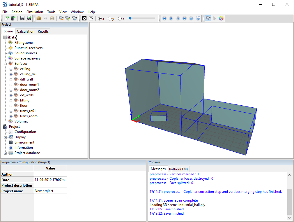
3D scene import in I-Simpa

Define a machine as a sound source

At this step, we want to create the sound sources. In industrial environments, sound sources are often machines or workstations made up of several source points. Since the hall can be made up of several identical machines located at different locations, it is simpler to define a machine in the form of a group of sound sources, which group can then be copied and moved within the room. In our example, we will define machines composed of three sound sources, which will be duplicated. Each sound source will be defined by a pink noise spectrum, with a global level of 80 dB.

1. Right-click the “Data/Sound Sources” element in the “Scene” tab of the “Project” windows, and Select “New Group”. By default, the name of the new group is “Sound sources”.

2. Rename the group as the following “Milling machine”;

3. Right-click on the “Milling Machine” group and select “New Source”. Perform this operation three times (to create three sources), named “Source 1”, “Source 2” and “Source 3”. It is possible to modify the name of the sources by applying the same method as for the name of a group;

4. For each source, Unfold the source properties, then Click on the “Position” item, and Assign the following coordinates (x,y,z) for the source 1 (2,7,1.2), the source 2 (2,6,0.6) and the source 3 (1,7,0.75).

5. For each source, Select the “Sound power” element, Choose “Pink Noise”, and then Set the global level “Lw” to 80dB.

Duplicate the machine

The previous machine can then be duplicated and moved into the room.

1. Right-click on the “Milling Machine” group and Select “Copy”;

2. Right-click the “Sound Sources” root folder, then Select “Paste”: an item named “Copy of Sound sources” is created.

Note

The sound sources within the new group have exactly the same properties as the original sources, including the names of the sources. However there is no possible confusion between two sources with the same name, each source having its own internal identifier.

3. Rename the group created in “Milling machine 2”;

4. Since the new machine is located in the same place as the original machine, it is necessary to move it. To perform a translation of the new machine, Right-click on the “Milling Machine 2” group and Select All sources ‣ Translation item menu;

5. Set the translation values in each direction (x,y,z) to [5,-2,0], and Click on “OK”. The sources group is translated.

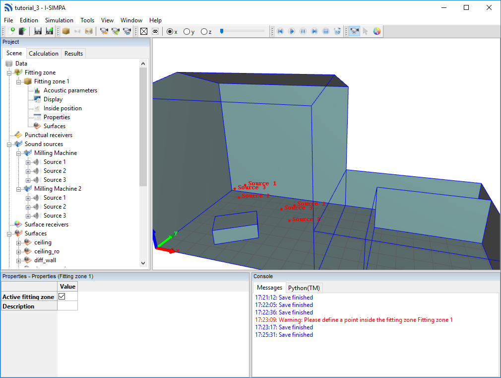
Sound sources creation (2 identical machines made of 3 punctual sources)

Define a scene volume as a fitting zone

There are two methods of creating a fitting zone in the room:

• when creating the scene with the CAD software. In this case, a closed volume is modeled in the 3D geometric model. It is then a “Scene fitted zone”

• either in I-Simpa, in the form of a parallelepipedal zone. It is then a “Rectangular fitted zone”

In our example, a parallelepipedal zone has already been provided at the creation of the 3D scene, in order to be assigned to a “Scene fitted zone”.

1. In the “Scene” tree, Right-click on the “Fitting zone” root folder and Select “Define scene fitted zone”;

2. Now you have to define the surfaces of the scene for the corresponding zone. Select the surface selection mode on the “Selection” toolbar; Hold Ctrl keyboard key and Double-click on each face element of the the fitting zone. Each face element is selected in red (or another color depending of the I-Simpa Settings). At the same time, the corresponding face elements are also highlighted in the folder “Surfaces” of the “Data” tree.

Note

Holding the Ctrl keyboard key allow to select all coplanar face element by a double click. You can also use the same procedure, but with one single click, to select each face element independently.

3. In the folder “Surfaces” of the “Data” tree, Select all highlighted face elements, and drag/drop them to the “Surfaces” element of the fiiting zone. All face elements are then duplicated in this folder.

Note

In this example, all face elements were already identified in a given folder “fitting” of the “Data” tree, because this volume was build when preparing the 3D geometry. In this case, it was not necessary to follow the step 2 of this procedure. One can directly drag and drop all face elements of the corresponding surface folder.

4. One must also select the face elements of the fitting zone that are located on the ground. Open the “floor” surface group and find the two face elements that correspond to the floor of the fitting zone (Select each face element of the group and Identify the ones that correspond to the fitting zone). Once the two face elements are identified, Select them and drag/drop them to the “Surfaces” element of the fitting zone.

5. Define the “Acoustic parameters” of the fitted zone, with 0.25 for “Alpha” (absorption coefficient of the obstacles), 0.5 m for “Lambda” (mean free path in the fitted zone) and “Uniform reflection”. See the SPPS documentation for more information about acoustic parameters of fitted zones.

Astuce

When you define value in a spreadsheet (for example “Alpha” in the example above), you can duplicate the value in all the column (i.e. frequency bands) by selecting :Set the same value ‣ To the column after a Right-Click on the corresponding value.

You can also define an average value by setting a value to “Average” (last row of the spreadsheet), which will define the same value for all the rows (i.e. frequency bands).

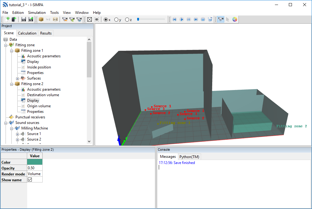
Fitting zones representation (scene and parallelipipedic fitting zones)

Define a parallelipipedic volume as a fitting zone

One may create a fitting zone as a parallelipipedic volume directly within I-Simpa. Such volume is defined by creating the two opposite corners of the volume. In the following example, one consider a fitting zone made of chairs.

1. Right-Click on the “Fitted zone” element of the “Data” tree, and Select “Define rectangular fitted zone”. A new fitted zone is created.

2. Define the “Position” element (coordinates) of the opposite corners of the fitting zone, “Origin volume” and “Destination volume”, as (13,4,0) and (18,1,1.2) respectively.

3. Define the “Acoustic parameters” of the fitted zone, with 0.15 for “Alpha” (absorption coefficient of the obstacles), 0.3 m for “Lambda” (mean free path in the fitted zone) and “Uniform reflection”.

Define surface materials

User can define specific material for the project.

1. Unfold the “Materials” element of the “Project database” element of the “Project” tree and Right-Click on the “User” element. Select “New material”. A “New material” is created. Rename the name of the corresponding material to “Trans_material”.

2. Select the “Material spectrum” element to display the acoustic parameters of the corresponding material. Set the values of each parameters according to the following table.

Acoustical properties of the “Trans_material” material

Frequency bands	Absorption	Diffusion	Transmission	Loss (dB)	Diffusion law
125 Hz	0.11	0.3	Check	10	Lambert
250 Hz	0.08	0.4	Check	11	Lambert
500 Hz	0.07	0.5	Check	12	Lambert
1000 Hz	0.06	0.6	Check	13	Lambert
2000 Hz	0.09	0.7	Check	14	Lambert
4000 Hz	0.05	0.8	Check	15	Lambert

3. Go to the “Surfaces” folder in the “Data” tree. Select the “trans_ro1” surface to display the coresponding “Properties” and set the “Material” parameter to the “Trans_material” material. Repeat this procedure for the “trans_room” surface group.

4. Create a new material “Open_door” using the same procedure as for “Trans_material”, using the following parameters, and Set this material to the “door_room1” and “door_room2” surface groups.

Acoustical properties of the “Open_door” material

Frequency bands	Absorption	Diffusion	Transmission	Loss (dB)	Diffusion law
125 Hz	1.0	0	Check	0	Can not be defined
250 Hz	1.0	0	Check	0	Can not be defined
500 Hz	1.0	0	Check	0	Can not be defined
1000 Hz	1.0	0	Check	0	Can not be defined
2000 Hz	1.0	0	Check	0	Can not be defined
“4000” Hz	1.0	0	Check	0	Can not be defined

5. For all other surfaces groups, Set the material to “30% absorbing” from the “Reference materials” database.

Astuce

For all these surface groups, since the surface material is the same, user can move all surface elements to a given surface group and set the material to this surface group only.

Note

The surface elements that have been defined as fitting surfaces (i.e. “fitting” surface group) are consider as perfeclty transparent by default. CAUTION

Astuce

In order to verify that material have been correctly set, you can display the 3D by selecting the “Material” option in the :View ‣ Material color menu.

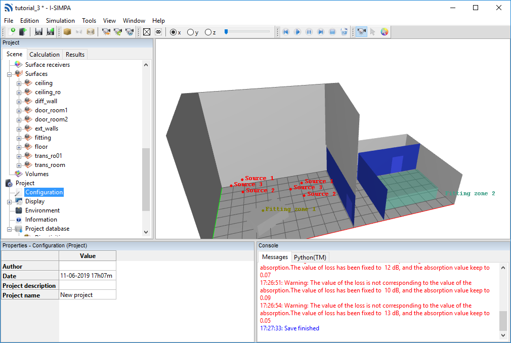
Representation of material of scene surfaces

Insert a line of punctual receivers

Instead of creating punctual receivers individually, you can directly create a line (or an grid) of punctual sound sources.

1. Go to the “Punctual receivers” folder in the “Data” tree and Right-Click on it. Thus, Select the “Create a receveir grid” option.

2. A spreadsheed is displayed to define the receiver grid parameters. See the corresponding documentation for more information concerning these parameters. Set the following values:

Receiver grid parameters

Parameter	Value
“Col step x (m)”	1
“Col step y (m)”	1
“Col step z (m)”	0
“Number of rows5	5
“Number of cols”	1
“Row step x (m)”	2
“Row step y (m)”	0
“Row step z (m)”	0
“Starting position x (m)”	0
“Starting position y (m)”	1
“Starting position z (m)”	1.6

Astuce

To create a grid of receivers instead of a line of receivers in the example above, change the value of the “Number of cols” parameter to 2 or more.

Define a plane receiver

1. Following the same procedure than for the Elmia tuturial, Create a “New plane receiver”, using the default parameters.

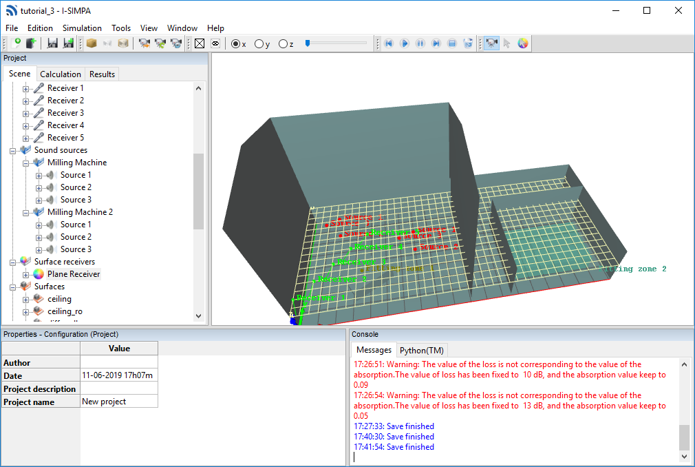
Line of punctual receivers (green) and plane surface receiver (mesh)

SPPS calculation

1. Go to the calculation tab of the “Project” windows, Unfold the “SPPS” code and Select the “Properties” element. It displays a spreadsheet with all SPPS calculation parameters.

2. Set the parameters to the corresponding values (see the correspondig documentation for more information about these parameters):

SPPS calculation parameters (tutorial 3)

Parameter	Value
“Active calculation of atmospheric absorption”	Check
“Active calculation of diffusion by fitting objects”	Check
“Active calculation of direct field only”	Uncheck
“Active calculation transmission”	Check
“Calculation method”	Energetic
“Echogram per source”	Uncheck
“Export surface receivers for each frequency band”	Uncheck
“Limit value of the particle extinction: ratio 10^n”	5
“Number of sound particles per source”	150 000
“Number of sound particles per source (display)”	0
“Random initialization number”	0
“Receiver radius (m)”	O.31
“Simulation length (s)”	2
“Surface receiver export”	Soundmap: SPL
“Time step (s)”	0.002

3. Right click the “Frequency bands” element and Select the option “Automatic selection”, “Octave”, “Building/Road [125-4000] Hz”.

4. Run the calculation code by right-clicking on the “SPPS” element and selecting “Run calculation”

Evaluate the effect of changing one surface material

One can be interesting to evaluate the effect of changing one surface material. I-Simpa includes a tool that allows to compare two results on a surface material. For such operation it is important that the surface receiver is not changed between the tow simulation.

1. Create a new material named “Aborbing_material” using the following data:

Acoustical properties of the “Absorbing_material” material

Frequency bands	Absorption	Diffusion	Transmission	Loss (dB)	Diffusion law
125 Hz	0.60	0	Uncheck	0	Specular
250 Hz	0.62	0	Uncheck	0	Specular
500 Hz	0.77	0	Uncheck	0	Specular
1000 Hz	0.74	0	Uncheck	0	Specular
2000 Hz	0.80	0	Uncheck	0	Specular
“4000” Hz	0.81	0	Uncheck	0	Specular

2. Set the “Diff_wall” surface to the new material “Absorbing_material”.

3. Run a new SPPS calculation using the same calculation parameters. At this step, two simulation results are available in the “Results” tab of the SPPS code.

4. Goto to Tools ‣ “File results process” ‣ “Compare surface receivers” menu

5. In the list, Select the data “rs_cut” in the “Surface receiver” ‣ “Global” list element of the surface receivers used as a “reference” (should be the first calculation, but you can choose the second calculation instead), then Select “Next”.

6. In the list, Select the data “rs_cut” in the “Surface receiver” ‣ “Global” list element of the surface receiver that must be compared to the reference (i.e. the “other simulation”, should be the second calculation, but you can choose the first calculation instead). At this step, you can defined a name for the difference between the two results (“reference” - “other simulation”) (by default “Power gain”) and create a new data file by checking the corresponding box. Then Select “Finish”. The corresponding result is created in the folder “Surface receiver” ‣ “Global” of the second result.

7. Right-click on the “Power gain” result and choose “Load animation” ‣ “Cumulating sound level” to display a sound map of the difference between the two results.

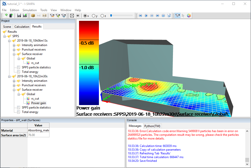
SPL sound map showing the difference between two calculations.