Modelling of physical phenomena in SPPS¶

Sound source modelling¶

General formalism¶

Acoustic directivity and probability density of sound particles emission¶

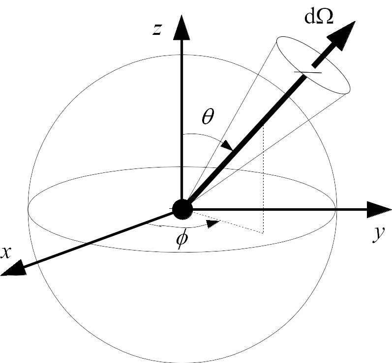
From a numerical modelling point of view, the problem of sound emission from a point source is to attribute to the sound particles, at a given moment (which can be the origin of time), the exact position of the source, propagation directions in accordance with the directivity of the source. For example, in the case of an omnidirectional sound source, it is necessary to verify that the sound particles, once emitted, are uniformly distributed over a sphere centred on the source (see corresponding figure: Elementary geometry for a sound source). The first solution that comes to mind is to make a deterministic discretization of the source’s radiation in spherical coordinates; the method would consist in considering emission angles $\theta$ and $\phi$ by constant steps. Nevertheless, such discretization of emission angles causes an artificial concentration of sound particles at the poles of the sphere symbolizing the source.

Elementary geometry for a sound source¶

The direction of emission of a particle is defined in spherical coordinates by the angles $\phi$ (azimuth) between $0$ and $2\pi$, and $\theta$ between $0$ and $\pi$ (polar angle), or by the elementary solid angle $d\Omega$.

It is in fact necessary to check the respect of the number of particles emitted by elementary solid angle $d\Omega = d\phi\,\sin\theta\,d\theta$, checks the directivity of the source, either in a deterministic or random way (figure[geo_source]). In our case, we chose a random draw of the initial directions of the particles. It is then necessary to define the probability densities $g(\phi)$ and $p(\theta)$, respectively for the angles $\phi\in[0.2\pi]$ and $\theta\in[0.\pi]$, such as the probability density $Q(\theta,\phi)$ of emission in the direction $(\theta,\phi)$ (or probability density $F(\Omega)$ of emission in the elementary solid angle $\Omega$) either in accordance with the directivity of the source. In practice, $Q(\theta,\phi)$ is nothing more than the directivity of the source. By definition, these probability densities verify the following relationship:

\[\begin{split}\begin{aligned} \int F(\Omega)\, d\Omega &= \iint Q(\theta,\phi) \,\sin\theta \, d\phi\,d\theta \\ &=\int_{0}^{2\pi} g(\phi) \, d\phi \int_{0}^{\pi} p(\theta)\,\sin\theta\,d\theta\\ &=1. \end{aligned}\end{split}\]

From the point of view of sound power, this is equivalent to considering that the power $W$ of the source is well distributed over the surface of a sphere centered on the source:

\[\iint W\,Q(\theta,\phi) \,\sin\theta \, d\phi\,d\theta=W.\]

If the densities $g(\phi)$ and $p(\theta)$ are independent, they check:

(1)¶\[\label{cond_g} \int_{0}^{2\pi} g(\phi) \, d\phi = 1,\]

and

(2)¶\[\label{cond_p} \int_{0}^{\pi} p(\theta)\,\sin\phi\,d\theta=1.\]

Source power and elementary particle energy¶

Acoustically, for a period of time $\Delta t$, a power source $W$ emits an amount of energy $E=W\times \Delta t$. From a particle concept point of view, each particle carries an elementary energy $\varepsilon_0$. If the source emits $N$ sound particles, the energy conservation between the two approaches therefore requires:

\[N \times \varepsilon_0 = W\times \Delta t,\]

then

\[\label{energie_elementaire} \varepsilon_0 = \frac{W}{N}\times \Delta t.\]

Omnidirectionnal source¶

Physical description¶

An omnidirectional sound source is a source that radiates in all directions with the same amplitude. The directivity of the source is similar to a sphere. The directivity coefficient $Q$ associated with the directivity of the source is equal to $1$.

Modeling¶

In the case of an omnidirectional source, the densities $g(\phi)$ and $p(\theta)$ being uniform, the relationships (1) and (2) verify:

\[\int_{0}^{2\pi} g(\phi) \, d\phi =\int_{0}^{2\pi} A \, d\phi = 1\]

and

\[\int_{0}^{\pi} p(\theta)\,\sin\theta\,d\theta=\int_{0}^{\pi} B\,\sin\theta\,d\theta=1,\]

where $A=1/2\pi$ and $B=1/2$ are two normalization constants. In practice, the method consists first of drawing an angle $\theta$ between $0$ and $2\pi$ as follows:

\[\label{choix_phi} \phi=2\pi \times u \quad \in [0,2\pi]\]

where $u$ is a random number between $0$ and $1$, and defined by a uniform distribution. If the angle $\theta$ is chosen in the same way (i.e. $\theta= \pi \times v$, $v$ being a random number with a uniform distribution between $0$ and $1$), the distribution of the emission directions does not respect the elementary solid angle consistency, since the condition ([cond_p]) is not verified. In this case, the directions around the poles would be preferred. It is actually necessary to determine the angles $\theta$ which verify a distribution proportional to $\sin\theta$. In this simple case, the procedure consists in applying the inverse cumulative distribution function method. According to the relationship (2), the probability $f(\hat{\theta})$ of drawing an angle $\theta<\hat{\theta}$ is given by:

\[\label{cdf_dist_theta} f(\hat{\theta}) = \frac{1}{2} \int_{0}^{\hat{\theta}} \sin\theta \, d\theta=\frac{1}{2} \left[\cos\hat{\theta}-1\right].\]

Knowing that this distribution is between $0$ and $1$, the choice of the angle $hat{\theta}$ is made by randomly drawing a number $v\in[0.1]$, following a uniform distribution, such as:

\[\hat{\theta} = \cos^{-1} \left(2v-1\right)\quad \in [0,\pi].\]

The propagation vectors $\mathbf{v}(v_x,v_y,v_z)$, of standard $c$ (sound velocity), are then defined by the relationships:

\[\begin{split}\mathbf{v}=\left\{\begin{array}{l} v_x=c\,\cos\theta\,\sin\phi\\ v_y=c\,\sin\theta\,\sin\phi\\ v_z=c\,\cos\phi \end{array}\right.\end{split}\]

Verification¶

The figures Distribution of emission angles \phi for an omnidirectional source and Distribution of emission angles \theta for an omnidirectional source shows an example of the distribution of angles $\theta$ and $\phi$ obtained according to this printing method with $10000$ achievements. It is easy to see that the angle distribution checks the theoretical distribution. It is understood that the quality of the random draw depends on the method of generating random numbers, and that compliance with theoretical distributions increases with the number of draws.

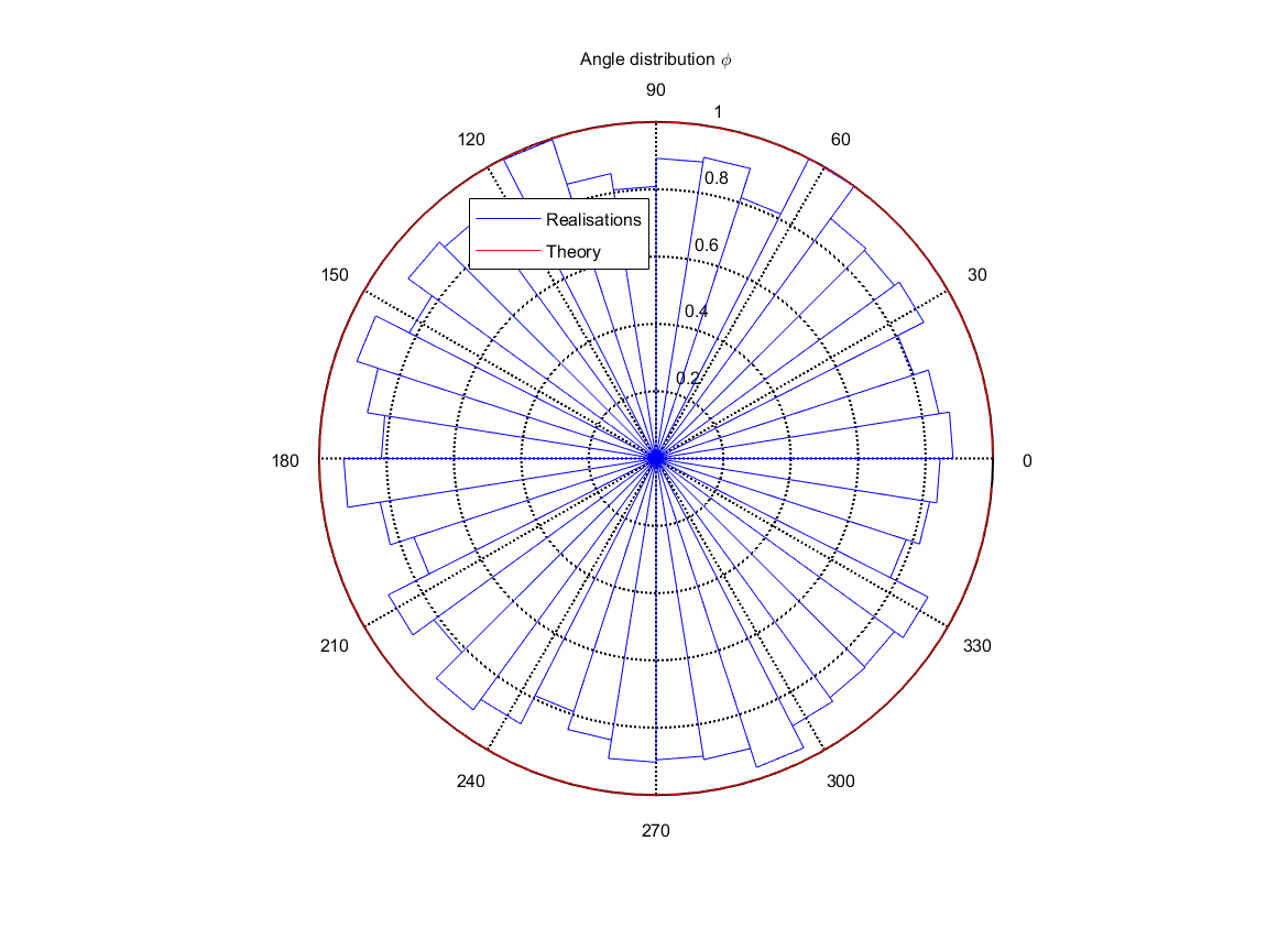
Distribution of emission angles for an omnidirectional source.

Distribution of emission angles $\phi$ for an omnidirectional source¶

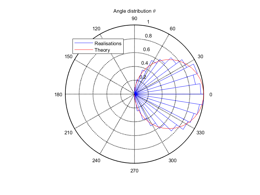
Distribution of emission angles $\theta$ for an omnidirectional source¶

Unidirectional source¶

Physical description¶

A unidirectional sound source is a source that radiates in a single direction of space, defined by the angles $\theta$ and $\phi$, at the point of emission and in the absolute reference point. The directivity coefficient associated with the directivity of the source is then defined by:

\[Q\left(\theta,\phi\right)=\delta\left(\theta,\phi\right)=\delta\left(\theta\right)\times\delta\left(\phi\right),\]

where $\delta$ is the Dirac distribution funtion.

Modelling¶

The modelling of this type of source is entirely deterministic and therefore does not pose a problem. It is enough to define a vector $\mathbf{s}(s_x,s_y,s_z)$ in the absolute reference frame of the scene, such that:

\[\begin{split}\mathbf{s}=\left\{\begin{array}{l} s_x=s\,\cos\theta\,\sin\phi\\ s_y=s\,\sin\theta\,\sin\phi\\ s_z=s\,\cos\phi \end{array}\right.\end{split}\]

Plane sources (XY, YZ and XZ)¶

Physical description¶

A “plane” type sound source is a source that radiates in a plane. By default, we consider three sources XY, YZ and XZ defined by the three reference planes $(xOy)$, $(yOz)$ and $(xOz)$ respectively.

Modelling¶

The procedure consists in randomly determining the direction of propagation of a particle in a plane. Using the angle convention presented in figure Elementary geometry for a sound source, we will have:

\[\begin{split}\left\{\begin{array}{llll} \text{XY plane:}& \theta=2\pi \times u\quad &\text{and}&\quad \phi=\pi/2\\ \text{YZ plane:}& \theta=0 \quad &\text{and}&\quad \phi=2\pi \times u\\ \text{XZ plane:}& \theta=\pi/2\quad &\text{and}&\quad \phi=2\pi \times u \end{array}\right.\end{split}\]

where $u$ refers to a random number between $0$ and $1$. Thereafter, the propagation vector $\mathbf{v}(v_x,v_y,v_y,v_z)$, of standard $c$ (sound velocity), is defined by the relationships:

\[\begin{split}\mathbf{v}=\left\{\begin{array}{l} v_x=c\,\cos\theta\,\sin\phi\\ v_y=c\,\sin\theta\,\sin\phi\\ v_z=c\,\cos\phi \end{array}\right.\end{split}\]

Acoustic propagation modelling¶

Acoustic propagation¶

Physical description¶

In the absence of absorption and reflection on the walls of the domain or on objects, the decrease in sound intensity from an omnidirectional source is written:

\[I=\frac{Q}{4\pi\,r^2},\]

where $r$ is the distance to the source, and $Q$ is the directivity of the source in the direction of observation ($Q=1$ for an omnidirectional source). This decrease reflects the phenomenon of geometric dispersion, which describes the « spreading » of a spherical wave as it propagates.

Modeling¶

Considering the method presented for an omnidirectional source, the geometric dispersion is automatically respected. Indeed, the proposed numerical method allows to obtain a uniform distribution of particles over an elementary solid angle. On a sphere, the particle distribution $n(r)$ (in $m^2$) is therefore equal to:

\[n(r)=\frac{N}{4\pi\,r^2},\]

where $N$ is the number of particles. The particle distribution therefore verifies the same decrease as the intensity. It should be noted, however, that the further away the observation point is from the source, the more sound particles will be required.

Verification¶

The figure Verification of the respect of the geometric dispersion with the SPPS code shows the numerical results of the free field propagation (the free field is simulated by considering a long corridor with perfectly absorbent limits), for an omnidirectional sound source, without atmospheric absorption (number of particles $N=20\times 10^6$). The agreement is excellent.

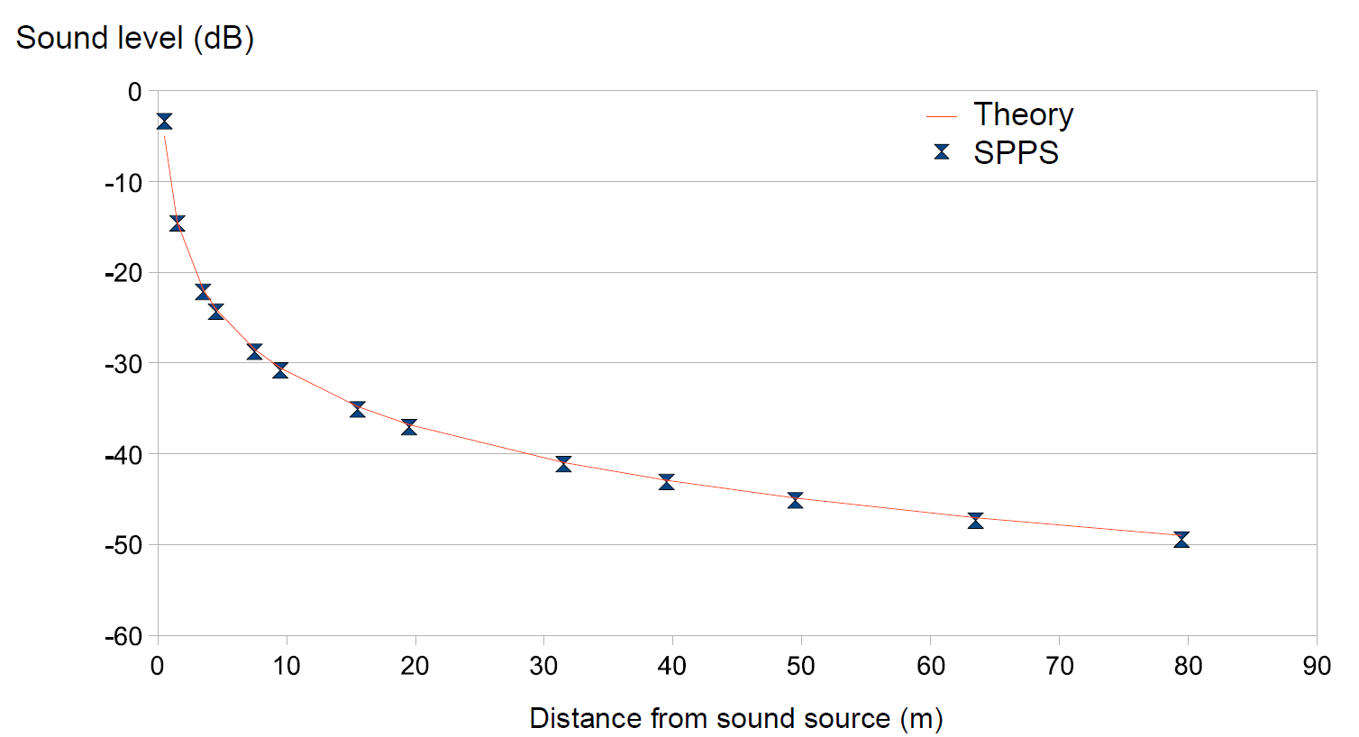
Verification of the respect of the geometric dispersion with the SPPS code¶

The numerical simulations are compared with the theoretical decrease ($N=20\times 10^6$ particles). The marker presents the result of the simulation with the SPPS code. The solid line shows the theoretical geometric dispersion.

Atmospheric absorption¶

Physical description¶

During its propagation in air, a sound wave is partially attenuated by particular physical mechanisms (« classical » transmission processes, molecular absorption due to rotational relaxation, molecular absorption due to vibratory relaxation of oxygen and nitrogen) [BSPE84]. Thus, after a propagation distance $r$, the amplitude $p_t$ of the sound pressure decreases according to the relationship (ISO 9613-1):

\[\label{eq:att_atmos_pression} p_t= p_i \exp \left(-\frac{\ln(10)}{20}\alpha_\text{air}\times r\right)\]

where $p_i$ is the initial pressure. Considering that the sound intensity is proportional to the square of the sound pressure,

\[\label{eq:att_atmos_pression_I} I\propto p_t^2 \propto \exp \left(-2\frac{\ln(10)}{20}\alpha_\text{air}\times r\right)\]

and writing that the intensity $I$ of the sound wave decreases with the relationship:

(3)¶\[\label{eq:att_atmos} I= I_0 \exp -m\,r,\]

where $I_0$ is the initial intensity of the sound wave. Then, the atmospheric absorption coefficient $m$ (in Np/m) can be expressed from the atmospheric absorption coefficient $\alpha_\text{air}$ (in dB/m), by the relationship:

\[m=\frac{\ln 10}{10}\alpha_\text{air}.\]

In SPPS code, the atmospheric absorption coefficient $\alpha_{air}$ is calculated according to ISO 9613-1, considering the centre frequency of each frequency band of calculation according to the reference standard (cf. paragraph 8.2.1 of ISO 9613-1). This approximation is considered valid if the product of the source-receiver distance (in km) by the square of the centre frequency (in kHz) does not exceed 6 km.kHz $^2$ for the third octave bands and 3 km.kHz $^2$ for the octave bands. However, the propagation distance must not exceed 6 km for third octave bands and 3 km for octave bands, regardless of the centre frequency considered.

Random modelling¶

By choosing the “random” calculation mode, atmospheric absorption is taken into account as a probability of the sound particle disappearing during its displacement. The corresponding probability density can be defined from the relationship (3):

\[f(r)=\exp -m\,r.\]

This quantity expresses the probability that the particle will not be absorbed during its propagation distance $r$. The probability density $f(r)$ is well between $1$ and $0$ (see figure Modelling of atmospheric absorption by a random process):

$f(0)=1$, the probability is maximum, the particle cannot be absorbed if it does not move;
$f(\infty)=0$, the probability is zero since the particle cannot spread infinitely.

It is also easily verified that the probability of propagation is independent of the previous probability of propagation:

\[f\left(\Sigma_{n=1}^N r_i\right)=\Pi_{i=1}^N f(r_n).\]

Taking atmospheric absorption into account is relatively simple. It is sufficient to consider a uniform random number $\zeta$ between $0$ and $1$, at each time step, and to compare this number to the probability density $f(d_0)$ corresponding to an elementary displacement $d_O=c\Delta t$ on a time step $\Delta t$. If this number $\zeta$ is less than $f(d_o)$, there will be propagation. Otherwise, there will be atmospheric absorption, thus disappearing the particle. Even on a small number of particles, this method makes it possible to correctly take into account atmospheric absorption.

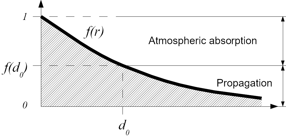
Modelling of atmospheric absorption by a random process¶

The curve $f(r)$ separates the propagation domain from the atmospheric absorption domain.

Energetic modelling¶

By choosing the “energetic” calculation option, the energy of the particle is weighted throughout its movement, using the relationship (3).

Verification¶

As an illustration, the figure Illustration of the modelling of atmospheric absorption in the SPPS code shows the sound decrease calculated by the SPPS code at $10$ kHz for classical atmospheric conditions ($T=20$ Celsisus, $H=50$ %, $P=101325$ Pa, or $m=0.036$ m $^{-1}$), for both types of modelling, compared to the theoretical decrease presented to the relationship (3); the simulation is identical to the one for the verification of the respect of the geometric dispersion.. As expected, energetic modelling gives a better result than random modelling, the average deviation from the theoretical curve being $0.17$ dB and $0.41$ dB respectively, the calculation times being similar.

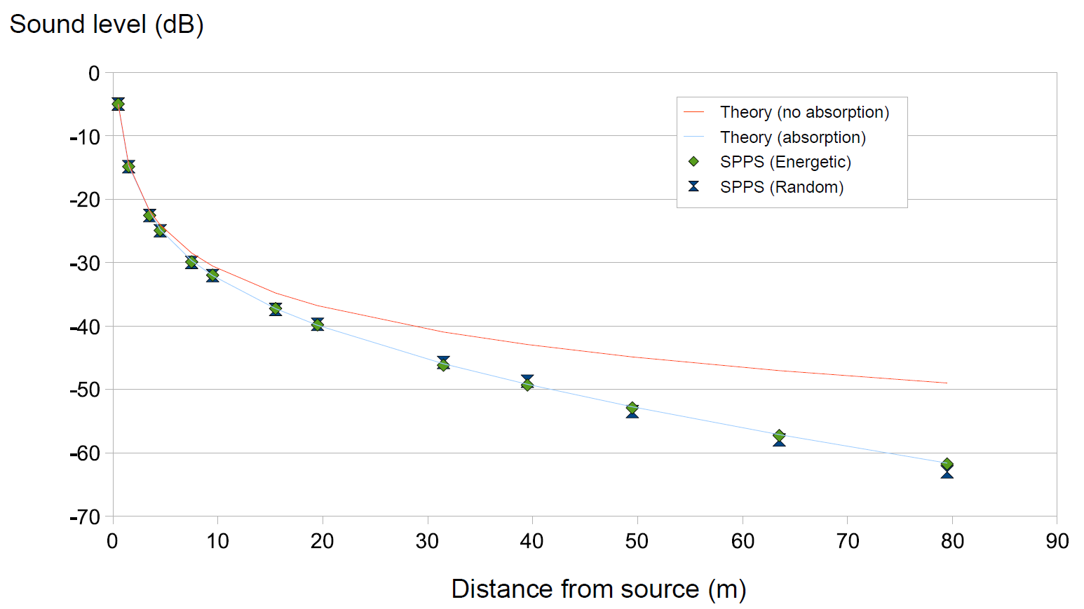
Illustration of the modelling of atmospheric absorption in the SPPS code¶

Comparison with the theoretical decrease (with et without atmospheric absorption) Simulations performed with ($N=20\times 10^6$ particles) at 10 kHz, for conventional atmospheric conditions: $T=20$ Celsisus, $H=50$ %, $P=101325$ Pa, or $m=0.036$ m $^{-1}$.

Acoustic velocity profile¶

Physical description¶

In outdoor environments, acoustic propagation can be influenced by micrometeorological conditions governed by thermal (heat transfer) and aerodynamic (wind profiles) laws. The phenomena have a very strong interaction with the ground (topography, surface and subsoil temperature, hygrometry, crops, forests, obstacles, buildings, etc.). In addition, they evolve rapidly in time and space, making their analytical description and numerical modelling complex. The thermal and aerodynamic factors that influence propagation are as follows:

Thermal factors: heat exchanges between the ground and the lower layer of the atmosphere lead to a variation in air temperature as a function of the height above the ground, and therefore to a variation in sound velocity.

Aerodynamic factors: due to the roughness of the ground surface, wind speed is always higher at height than at ground level. In a given situation, the speed of sound in the presence of wind corresponds to the algebraic sum of the speed of sound in the absence of wind and the projection of the wind vector on the direction of propagation considered. This speed therefore varies according to the height above the ground.

By analogy with the laws of optics (see figure Schematic representation of the acoustic refraction in the atmosphere in the presence of a vertical velocity profile), the effect of atmospheric conditions on acoustic propagation can be described through the expression of the acoustic index $n$ of the propagation medium. If placed in a vertical section, this index is assumed to vary with altitude $z$ and with source-receptor distance $r$, such that:

\[n(r,z)=\frac{c(r,z)}{c_0}=\langle n(r,z)\rangle + \mu(r,z),\]

where $c$ the reference one. Thus, two distinct phenomena can be distinguished that affect acoustic propagation, refraction and atmospheric turbulence. These phenomena are respectively related to the deterministic parts $\langle n\rangle$ and stochastic $\mu$ of the propagation medium index. In practice, these refraction and turbulence phenomena co-exist and interact, leading to complex propagation conditions, as well as a very wide dispersion of the sound levels encountered in situ, all of which are identical (topography, soil type, source-receptor geometry, etc.).

$Schematic representation of the acoustic refraction in the atmosphere in the presence of a vertical velocity profile.$

Schematic representation of the acoustic refraction in the atmosphere in the presence of a vertical velocity profile¶

Acoustic velocity profile model¶

The average sound velocity profile thus depends on the average wind and temperature profiles. This velocity profile can be described analytically, depending on whether it follows a linear (« $\text{lin}$ »), logarithmic (« $\text{log}$ »), hybrid (« $\text{log-lin}$ ») or other law. The « $\text{log}$ » profiles thus have the advantage of translating the very strong vertical gradient of sound velocity in the immediate vicinity of the ground, but do not accurately reflect the more moderate evolution with altitude above a certain height. On the other hand, the « $\text{lin}$ » profile minimizes the effects in the vicinity of the ground and are therefore not representative of reality when placed at very low altitude. A good compromise therefore consists in using hybrid profiles of the type « $\text{log-lin}$ » (valid especially for a so-called « stable » atmosphere), expressed through the parameters $a_\text{log}$ and $b_\text{lin}$ which appear in the analytical expression of the vertical profile of the effective sound velocity:

(4)¶\[\label{eq:celerite_log_lin} \langle c(z)\rangle=c_0+ a_\text{log}\times \ln\left(1+\frac{z}{z_0}\right)+b_\text{lin}\times \left( z-z_0\right),\]

où $z_0$ is the roughness parameter, whose typical values range from $10^{-2}$ m for short grass to several meters in urban areas. The vertical gradient is then expressed by deriving according to the variable $z$:

\[\frac{\partial\langle c(z)\rangle}{\partial z}=\frac{a_\text{log}}{z_0}+b_\text{lin}.\]

The main effect of propagation in a medium of variable speed is to bend the sound rays downwards or upwards depending on whether the vertical gradient of sound velocity is positive (conditions (very) favorable to propagation) or negative (conditions (very) unfavorable to propagation) respectively. The transient state between these two states represents homogeneous propagation conditions.

Homogeneous: the speed $c$ is the same at any point in the domain and equal to the reference speed $c_0$, the latter being calculated as a function of temperature and humidity conditions by the formula:

\[c_0=343.2\sqrt{\frac{T}{T_\text{ref}}},\]

where $T$ is the temperature (K), and $T_\text{ref}=293.15$ K the reference temperature (ISO 9613-1).

Very unfavorable : $a_\text{log}=-1$ and $b_\text{lin}=-0.12$;

Unfavorable : $a_\text{log}=-0.4$ and $b_\text{lin}=-0.04$;

Favorable: $a_\text{log}=+0.4$ and $b_\text{lin}=+0.04$;

Very favorable: $a_\text{log}=+1$ and $b_\text{lin}=+0.12$.

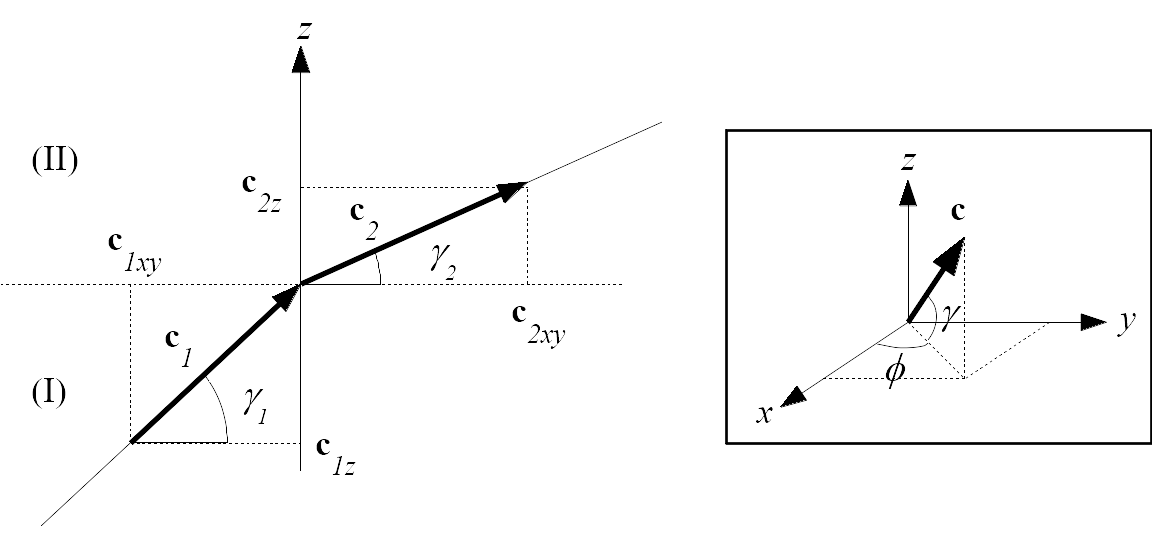
The curvature of the radius, at the boundary of zones (I) and (II), is obtained by applying the Huygens-Fresnel construction, resulting in the following Snell-Descartes law [Sal01] (see figure Schematic representation of the acoustic refraction in the atmosphere in the presence of a vertical velocity profile):

(5)¶\[\label{relation_snell} \frac{\cos\gamma_1}{c_1}=\frac{\cos\gamma_2}{c_2},\]

where $c_1$ and $c_2$ are respectively the norms of the propagation vectors $\mathbf{c_1}$ and $\mathbf{c_2}$, and where the angles $\gamma_1$ and $\gamma_2$ are defined with respect to the horizontal axis in the plane $(xOy)$. By construction, the projection of the propagation direction in the plane $(xOy)$, defined by the angle $\phi$ in spherical coordinates, is preserved.

Modelling¶

Whatever the method of calculation chosen, the speed is taken into account is identical. At each time step, the speed standard is calculated according to the chosen speed profile, based on the relationship (4). To determine the new direction of propagation, due to the change in speed, the relationship (5) must then be applied. Knowing the angle $\theta_1$ of the initial propagation direction, the new propagation direction is defined by:

(6)¶\[\label{cosgamma2} \cos\gamma_2=\frac{c_2}{c_1}\cos\gamma_1=\frac{c_2}{c_1}\frac{\sqrt{c_{1x}^2+c_{1y}^2}}{c_1}.\]

The coordinates of the propagation vector are then obtained by:

\[\begin{split}\mathbf{c_2}=\left\{\begin{array}{l} c_{2x}=c_2\cos\gamma_2\cos\phi\\ c_{2y}=c_2\cos\gamma_2\sin\phi\\ c_{2z}=c_2\sin\gamma_2 \end{array}\right.\end{split}\]

with

\[\sin\phi=\frac{c_{1y}}{\sqrt{c_{1x}^2+c_{1y}^2}},\]

and

\[\cos\phi=\frac{c_{1x}}{\sqrt{c_{1x}^2+c_{1y}^2}}.\]

From a numerical simulation point of view, the calculation of $\cos\gamma_2$ by the relationship (6) can give values higher than $1$ which is obviously not physical. This case occurs when the curvature (turning point) of a radius is reversed. To avoid this problem and impose a change in curvature, the procedure consists in imposing the value from $\gamma_2$ to $1-\epsilon$ ($\epsilon$ being a very small value) and changing the orientation of the component $c_{2z}$.

As an example, the figure [illustration_refraction] shows two illustrations of how acoustic refraction is taken into account using this method. This figure can be compared directly with the examples given in the reference [Sal01] (figures 4.5 and 4.6).

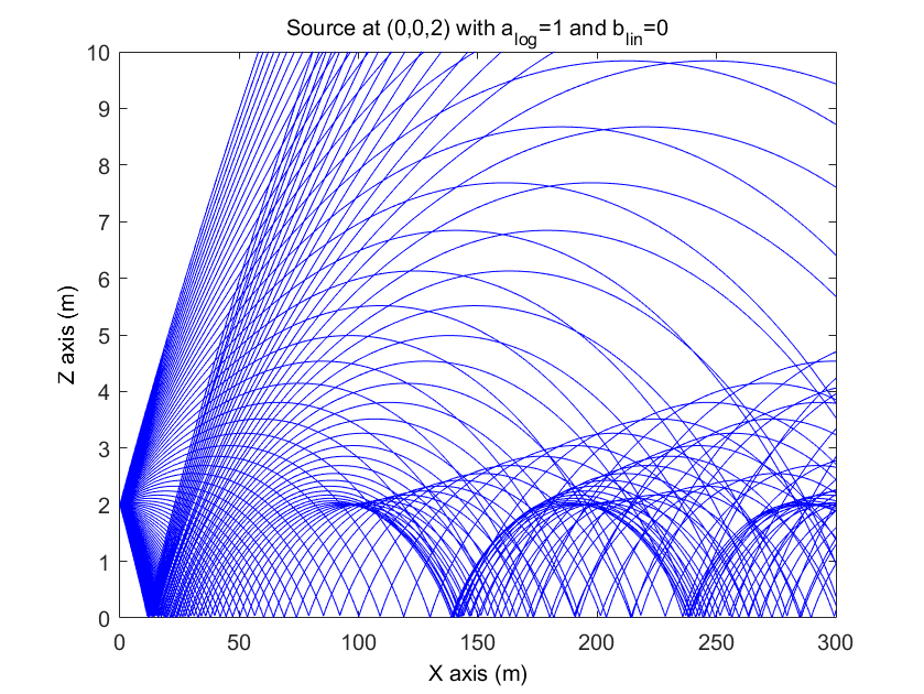
$Illustration of the modelling of acoustic refraction with SPPS in downward condition.$

Illustration of the modelling of acoustic refraction with SPPS in downward condition¶

$Illustration of the modelling of acoustic refraction with SPPS in upward condition.$

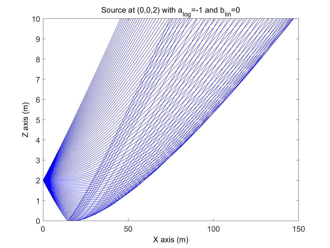
Illustration of the modelling of acoustic refraction with SPPS in upward condition¶

Diffusion by fittings¶

The presence of a large number of objects on the path of a sound wave can lead to a diffusion process. This process can be simulated in a deterministic way, by modelling each object individually. When the number of objects becomes large, and these objects are of similar sizes (example of an industrial hall with many machines (without acoustic emission) or similar boxes), it may be more interesting to statistically model this fitting zone.

Physical description¶

In order to take into account the diffusion and absorption of diffusing (or scattering) objects distributed in the propagation medium, we considered an approach similar to that of Ondet and Barbry [OB89], which itself is based on the work of many authors [Kut81][Aul85][Aul86][Lin82], among others. In this approach,

the diffusing objects (or obstacles, or fittings, or scattering objects…) are considered as punctual. Sound particles are returned in all directions of space at each collision with a scattering object (except in the case of absorption). This assumption is generally valid when the wavelength is in the order of magnitude of the characteristic dimension of the obstacle;
the scattering phenomenon follows a Poisson process, which means that the probability of collision of a sound particle with a scattering object follows a Poisson’s law. The collision probabilities are independent of each other (the collision probability during time $t$ and $t+dt$ is independent of collisions before time $t$);
the objects in the fitting zone do not produce particles (i.e. these objects are not sound sources).

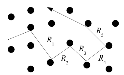
Schematic representation of the acoustic diffusion by obstacles in a fitting zone¶

A sound wave propagating in the environment may come into contact with scattering objects, causing the wave to diffract simultaneously and, in part, to absorb it. By analogy, in the particle approach, a particle that comes into contact with a scattering object can either be absorbed or reflected in another direction of propagation (see figure: Schematic representation of the acoustic diffusion by obstacles in a fitting zone). At the macroscopic scale, i.e. considering all the sound particles simultaneously, a diffusion process occurs, characterized by:

the absorption coefficient $\alpha_c$ of the scattering objects;
the bulk density $n_c$ of the propagation medium, defined by the number $N_c$ of obstacles present in the volume $V_c$:

\[n_c=\frac{N_c}{V_c}.\]

the average scattering section $q_c$, i.e. the average surface of the scattering object, seen by a particle in a given incident direction. In practice, this data is very difficult to obtain, if not impossible, since the scattering objects are of complex and different shapes. In this condition, it is common to assimilate the diffusing object to a sphere, having the same external surface $s_c$ as the object. Whatever the angle of incidence, the visible cross-section of the sphere (mean scattering cross-section) will be equal to a quarter of the total surface area of the sphere, or:

\[q_c=\frac{s_c}{4}.\]

the average diffraction section per unit volume $\nu_c$, also called the diffusion frequency, by

\[\nu_c=n_c\,q_c,\]

– if all the scattering objects are identical, or

\[\nu_c=\frac{1}{V}\sum_{p=1}^{N_c}\frac{s_{c_p}}{4}\]

– if each object diffusing $p$ is defined by its surface $s_{c_p}$. In practice, and in the rest of the document, the diffusing objects will be considered uniform in the same volume of diffusion. Nevertheless, within the same propagation volume, several separate diffusion volumes can be considered.

Since the scattering phenomenon follows a Poisson’s law, the probability that a sound particle will collide with scattering objects after a time $t_k$ is equal to:

\[W_k (c\,t_k)=\frac{\left(\nu_c \, c\,t_k\right)^k}{k!}\exp\left(-\nu_c\, c\, t_k\right),\]

where $c\, t_k$ is the distance covered during a time $t_k$, which can be expressed from the distance $R_p$ between two collisions (see figure: Schematic representation of the acoustic diffusion by obstacles in a fitting zone):

\[c\,t_k=\sum_{p=1}^k R_p.\]

Since the collision probabilities are independent of each other [OB89], it is easy to show that the random variables $R_i$ (noted $R$ afterwards) follow the following probability density $f(R)$:

(7)¶\[\label{dispois} f(R)=\nu_c \exp\left(-\nu_c \, R\right).\]

The average free path $\lambda_c$ (average distance between two collisions) is simply obtained by expressing the first moment of the above probability density, namely:

\[\lambda_c=\int_0^\infty R\, f(R)\, dR=\frac{1}{\nu_c}.\]

Modelling¶

By definition, the cumulative distribution function, associated with this probability density, is defined by the following relationship:

(8)¶\[\label{fdc} p(\hat{R})=\int_0^{\hat{R}} f(R)\, dR=1-\exp\left(-\nu_c\,\hat{R}\right).\]

This cumulative distribution function simply expresses the probability that the particle will collide with a scattering object during a long path $\hat{R}$. This function is therefore null for $\hat{R}=0$ and equal to $1$ for $\hat{R}=\infty$. The numerical simulation of the diffusion process is performed by the inverse cumulative distribution function method, obtained by reversing the relationship (8) , i.e.:

(9)¶\[\label{fdci} \hat{R}=-\frac{1}{\nu_c}\ln \left[ 1-p(\hat{R})\right].\]

The cumulative distribution function being between $0$ and $1$, it can be assimilated to a random variable $\xi$ between $0$ and $1$. By drawing a succession of random variables $\xi_i$, we can determine a succession of paths of length $\hat{R}_i$ that satisfies the distribution function (7) of our problem:

\[\label{fdci_2} \hat{R}_n=-\frac{1}{\nu_c}\ln \left[ 1-\xi_n\right].\]

An example of a random draw using the inverse cumulative distribution method is shown in Figure [fig:verification_diffusion_encrowding]. The comparison with the theoretical distribution shows an excellent behaviour of the method.

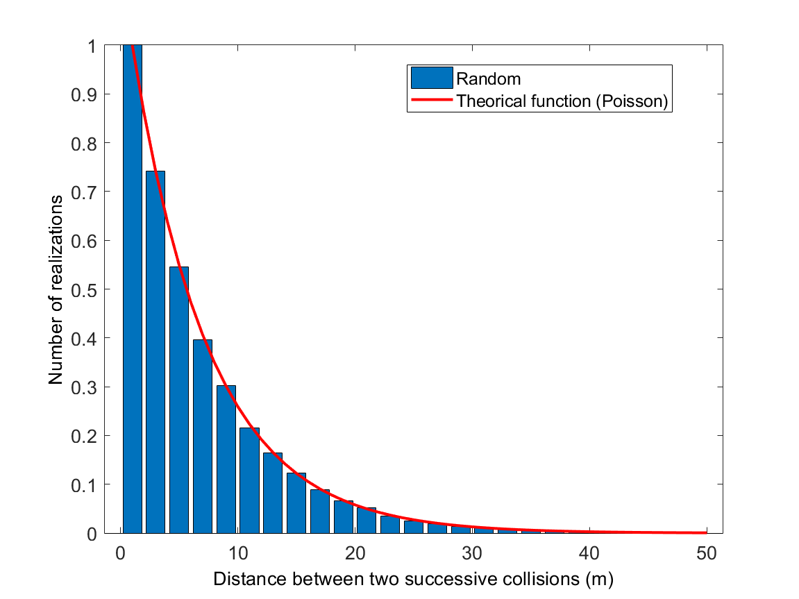
Distribution of the distance between two collission obtained by the inverse cumulative distribution function method and comparison with the theoretical distribution.

Distribution of the $\hat{R}_i$ paths obtained by the inverse cumulative distribution function method and comparison with the theoretical distribution¶

When a sound particle $n$ enters a fitting zone, it is associated with a collision distance $R_n$ with an object of the congestion by applying the relationship (9). As the sound particle propagates in the crowded area, a test is performed to determine if the cumulative distance $d_n$ of the particle in the crowded area is less or more than $R_n$. If the distance traveled $d_n$ is greater than the collision distance $R_n$ the particle collides with an object. In the “Energetic” mode, the energy of the sound particle is weighted by the average absorption coefficient $\alpha_c$ of the space requirement and continues its propagation in a random direction (uniform distribution). In the “Random” mode, a new random draw on a uniform variable $u$ allows to determine if the particle is absorbed by the diffusing object (same procedure than for considering absorption by a wall), or reflected in a uniform direction. After each collision, the cumulative propagation distance is reset to zero, and a new draw is made to determine the next collision distance. Whatever the calculation mode chosen, as long as the distance travelled by the particle is less than the collision distance, the particle continues its path without changing direction.

Wall modelling¶

Physical description¶

Absorption, dissipation and acoustic transmission¶

In contact with a wall (see figure Illustration of the mechanisms of reflection, absorption, dissipation (internal loss) and acoustic transmission through a wall), a sound wave will be partly reflected back into the domain for one part $R$, partly dissipated by transforming the acoustic energy into heat in the material for the other part $\beta$), the rest being transmitted through the material in the adjacent domain for the other par $\tau$. The latter coefficient is defined as the transmission factor. If $W_i$ is the power incident on a wall, then a part $W_r=R\,W_i$ will be reflected, a part $W_d=\beta\,W_i$ will be dissipated in the material, and a part $W_t=\tau\,W_i$ will be transmitted through the partition. By construction (there can be no creation of energy, nor more absorption than incident energy), the coefficients $R$, $\beta$ and $\tau$ are between 0 and 1, so the energy balance of the wall is written:

\[R+\beta+\tau=1.\]

Illustration of the mechanisms of reflection, absorption, dissipation and acoustic transmission through a wall.

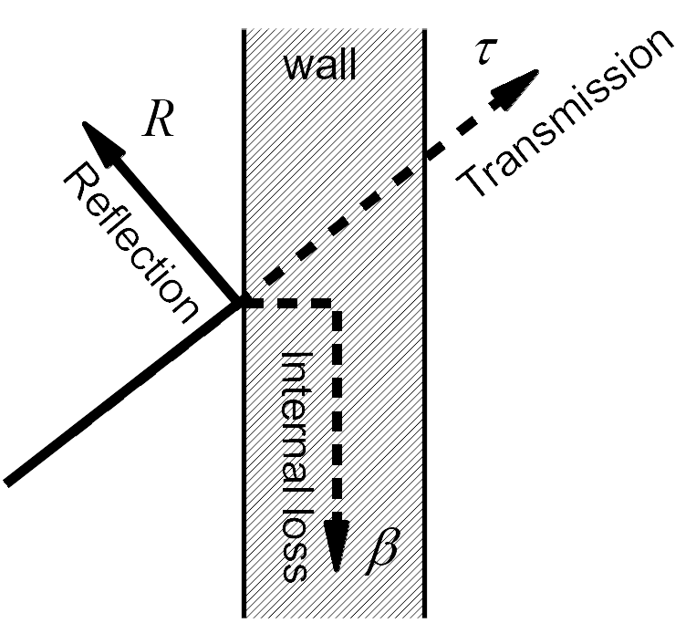
Illustration of the mechanisms of reflection, absorption, dissipation (internal loss) and acoustic transmission through a wall¶

It is usual to define the absorption coefficient $\alpha$ of the wall as the sum of the transmitted part $\tau$ and the dissipated part (internal loss) $\beta$, in the form $\alpha=\beta+\tau$, so that the above energy balance is written:

\[R=1-\alpha.\]

The absorption coefficient of a material can be measured using the standardised procedures ISO 354 for the reverberation chamber method, as well as ISO 10534-1 and ISO 10534-2 for the impedance tube method. For the sound transmission coefficient, the reader may refer to the different parts of the standards for air transmission (ISO 140).

Acoustic diffusion¶

On the other hand, depending on the shape, size and distribution of the wall irregularities, the sound wave can be reflected simultaneously in the specular direction and in other directions. In room acoustics, it is common to consider that a fraction $1-s$ of the sound energy will be reflected in the direction of specular reflection, while a fraction $s$ of the energy will be reflected in the other directions of space, according to a law of reflection characterized by irregularities in the wall [EAS01]. In the latter case, we speak of diffuse reflection, where $s$ is called scattering coefficient.

In room acoustics, numerous theoretical and experimental studies are currently underway to characterize or measure these laws of reflection [VM00][CDAntonio16]. However, the common practice is to use Lambert’s law to describe a diffuse reflection. The value of the scattering coefficient $s$ can be obtained by a standardized measurement procedure (ISO 17497-1).

Note

It is important to note that this scattering coefficient (ISO 17497-1), which defines the ratio between non-specular reflected energy on the total energy, is different from the diffusion coefficient $\delta$ (ISO 17497-2), which defines the ability of the surface to uniformly scatter in all direction. In some acoustic simulation software, the diffraction coefficient $s$ may sometimes wrongly called the diffusion coefficient.

Acoustic reflection modelling¶

Random modelling¶

First, a sound particle colliding with a wall can either be absorbed by the wall (with a probability $\alpha$), or reflected in a new direction of propagation (with a probability $R=1-\alpha$). In practice, the absorption/reflection choice is made by randomly drawing a number $u$ between $0$ and $1$, following a uniform distribution:

If this number is less than $\alpha=1-R$ (at the considered point), the particle is absorbed and disappears from the propagation medium.
If this number is greater than $\alpha=1-R$, the particle is reflected and continues to propagate in a new direction. In this last case, to determine the type of reflection (specular or diffuse), a new random draw $v$ is performed between $0$ and $1$:

– If this number is less than the value of $1-s$ (i.e. $v<(1-s)$) at the point considered, the particle is specularly reflected, in accordance with the well-known Snell-Descartes laws.

—Otherwise (i.e. if $v>(1-s)$), the reflection is diffuse. In the latter case, it is necessary to determine the direction of diffuse reflection.

Energetic modelling¶

When a particle collides with a wall, its energy $\epsilon$ is weighted by the reflection coefficient $R=1-\alpha$. The choice of specular or diffuse reflection, depending on the scattering coefficient, is identical to the “Random” method: a random draw $v$ is performed between $0$ and $1$. If this number is less than the value of $1-s$, the particle is specularly reflected. Otherwise, the reflection is diffuse, in a direction to be determined. An entirely “Energetic” treatment would be possible by duplicating the particle into two particles, the first being reflected in the specular direction and the second in the diffuse direction; however this last solution is not yet implemented in the SPPS code..

Modelling of the reflection laws¶

Formalism¶

Let us consider an incident sound particle on a wall, whose incident direction is defined by the spherical coordinates $(\theta,\phi)$ (see figure Elementary geometry of a reflection by a wall). This particle has a probability of $P(\theta,\phi;\theta',\phi')\equiv P(\Omega,\Omega')$ being reflected in the elementary solid angle $d\Omega' =\sin\phi'\, d\phi'\, d\phi'\, d\theta'$ [Joy74][Joy75][Joy78][LP03].

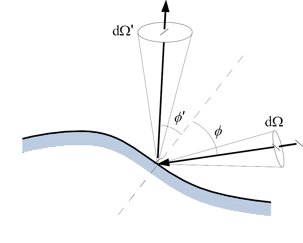
Elementary geometry of a reflection by a wall¶

Variables $\phi$ and $\phi'$ refer respectively to the angles of incidence and reflection with respect to the normal at the wall. The angles $\theta$ and $\theta'$ in the tangent plane, directions of incidence and reflection, are not represented ($\phi,\phi'\in[0,\pi/2]$ and $\theta,\theta'\in[0,2\pi]$).

$P(\Omega,\Omega')\,d\Omega'$ actually represents the fraction of the incident sound intensity that is reflected in the solid angle $d\Omega'$. Let’s say $j(\theta,\phi)$ the incident flow of particles. The flow of reflected particles $j'(\theta',\phi')$ is expressed:

(10)¶\[\label{eq_flux_1} j'(\theta',\phi') \cos \phi'=\int P(\theta,\phi;\theta',\phi')\, j(\theta,\phi) \cos \phi \,d\Omega.\]

Defining the reflection law $R(\theta,\phi;\theta',\phi')\equiv R(\Omega,\Omega')$ on the following:

\[R(\theta,\phi;\theta',\phi')=\frac{P(\theta,\phi;\theta',\phi')}{\cos(\phi')},\]

the relation (10) can be written:

\[\label{eq_flux_1b} j'(\theta',\phi') =\int R(\theta,\phi;\theta',\phi')\, j(\theta,\phi) \cos \phi \,d\Omega.\]

It is important to emphasize the difference between the law of reflection $R$ and the probability $P$. $P$ refers to a probability of reflection of a sound particle by elementary solid angle, while $R$ refers to the flow of energy reflected in a direction $\phi'$, for an incident flow in the direction $\phi$.

The first law of thermodynamics requires the conservation of the flow on the surface (in the absence of absorption). The law of reflection $R(\Omega,\Omega')$ must therefore check the following condition:

\[\label{loi_2} \int P(\Omega,\Omega') \,d\Omega'=\int R(\Omega,\Omega')\cos\phi' \,d\Omega'=1,\]

or, in spherical coordinates,

\[\label{loi_2b} \iint R(\theta,\phi;\theta',\phi')\cos\phi' \,\sin\phi'\,d\phi'\,d\theta'=1.\]

The second law of thermodynamics imposes this time:

(11)¶\[\label{loi_1} \int P(\Omega,\Omega') \,d\Omega=\int R(\Omega,\Omega')\cos\phi \,d\Omega=1,\]

or, in spherical coordinates,

(12)¶\[\label{loi_1b} \iint R(\theta,\phi;\theta',\phi')\cos\phi \,\sin\phi\,d\phi\,d\theta=1.\]

On the other hand, the principle of reciprocity requires that

(13)¶\[\label{loi_3} R(\Omega,\Omega')=R(\Omega',\Omega).\]

Despite some recent studies, and apart from Lambert’s law widely used to model diffuse reflections [Kut16], to our knowledge there are no other laws of reflection for real walls. In the SPPS code, however, we propose arbitrary modes of reflection, more or less real, presented in figure Illustration of the reflection laws proposed in the SPPS code.

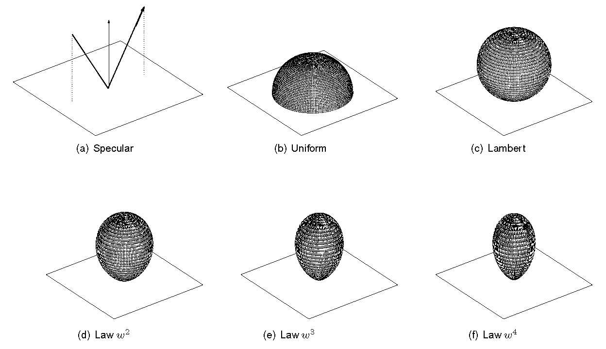
Illustration of the reflection laws proposed in the SPPS code¶

Specular reflection¶

Physical description¶

The simplest mode of reflection is defined by specular reflection and can be written in three dimensions:

\[R(\theta,\phi;\theta',\phi')=2 \delta(\theta-\theta' \pm \pi) \,\delta(\sin^2 \phi-\sin^2 \phi'),\]

where the couples $(\theta,\phi)$ and $(\theta',\phi')$ refer respectively to the incident and reflected directions of the sound particles on the wall. Although the form of this expression is not conventional, this relationship verifies the laws of Snell-Descartes, as well as the conditions (11) to (13).

Modelling¶

From a numerical point of view, the simulation of this reflection law does not pose a major problem, since the angles of incidence of each particle on a wall are known. The modelling is identical for the “Random” and “Energetic” »” approaches.

Uniform reflection¶

Physical description¶

A uniform reflection law produces a distribution of reflection angles $P(\Omega')$ that is equiprobable. This should not be confused with Lambert’s law of reflection, for which uniformity is verified by the law of reflection. In the case of a uniform law, particles are reflected uniformly throughout the half space, regardless of the angle of incidence. Under these conditions, the reflection density after normalization is written:

\[P(\Omega')d\Omega'= P(\theta',\phi')d\Omega'=\left[\frac{1}{2\pi}\,d\theta'\right] \,\left[\sin \phi' \,d\phi'\right],\]

or

\[R(\theta',\phi')=\frac{1}{2\pi\cos\phi'},\]

with $\theta'\in[0,2\pi]$ and $\phi'\in[0,\pi/2]$.

Modelling¶

From a numerical point of view, the determination of the angle of reflection is again obtained by the inverse cumulative distribution function method,

\[f(\hat{\phi})= \int_{0}^{\hat{\phi}} \sin\phi'\,d\phi'=1-\cos\hat{\phi},\]

which gives

\[\hat{\phi}=\cos^{-1}\left(1-u\right),\]

where $u$ is a random number between $0$ and $1$.

Lambert reflection¶

Physical description¶

In optics, a perfectly diffuse surface is a surface that also appears bright regardless of the angle of observation, and regardless of the angle of incidence. In terms of acoustics, a perfectly diffuse surface will reflect the same energy in all directions regardless of the angle of incidence. From a mathematical point of view, this condition requires that the law of reflection $R$ be independent of the direction of reflection, and therefore of the direction of incidence (by reciprocity). After normalization, the law of reflection is written:

\[R(\theta,\phi;\theta',\phi')=\frac{1}{2\pi}\times 2.\]

The coefficient $1/2\pi$ is related to the normalization according to the angle $\theta'$ (uniform distribution between $0$ and $2\pi$). The second coefficient (factor $2$) is related to the normalization according to the angle $\phi'$. The probability of $P(\Omega') d\Omega'$ is therefore reduced to

\[\begin{split}\begin{aligned} P(\Omega') \, d\Omega' & = R\,\cos\phi'\,\sin\phi'\,d\theta'\,d\phi'\\ & = \left[\frac{1}{2\pi}\,d\theta'\right]\, \left[2 \cos\phi'\,\sin\phi'\,d\phi'\right], \end{aligned}\end{split}\]

where the expression $\cos\phi'$ is related to Lambert’s law. It is easy to check that $R$ checks the conditions (11) to (13). It is important to note the difference between a random surface and an uniform surface. The first one is conditioned by an uniform random reflection law $R$, while the second is defined by a uniform probability $P$.

Modelling¶

From a numerical point of view, the random drawing of the reflection angles (in three dimensions) must be carried out in accordance with the distribution $P(\Omega')$, i.e. $P(\phi')$ in our case. Applying the inverse cumulative distribution function method, the probability $f(\hat{\phi})$ that a sound particle is reflected in an angle $\phi'$ between $0$ and $\hat{\phi}$ is given by the following relationship:

\[f(\hat{\phi})=2\int_{0}^{\hat{\phi}} \cos\phi'\sin\phi'\,d\phi'=\sin^2 \hat{\phi}.\]

Since this probability is between $0$ and $1$, the choice of angle $\hat{\phi}$ is made by randomly drawing a number $u\in[0.1]$, such that:

\[\hat{\phi}=\sin^{-1}\sqrt{u}=\cos^{-1}\left(1-u\right)^\frac{1}{2}.\]

Avertissement

It is important to note that other authors [BMC90][Hod91][Lam96][XKaJ02] mention other relationships. The correct formulation depends on the angle convention. It is also possible that some of the relationships that are proposed may not be accurate.

Normal reflection¶

Physical description¶

Let us consider a law of reflection independent of the incident direction and defined only by the angle of reflection $\phi'$ around the normal to the wall ($\theta'$ being uniform between $0$ and $2\pi$), of the form:

\[\begin{split}\begin{aligned} R(\Omega')&=R(\theta',\phi')\\ &=\frac{1}{2\pi}\times (n+1)\cos^{n-1}\phi'\\ &=\frac{n+1}{2\pi}\,w^{n-1}. \end{aligned}\end{split}\]

where $n$ is a positive integer. The quantity noted $w=\cos\phi'$ is none other than the projection of the direction of reflection on the normal at the wall. According to the notations in this document, the probability $P$ will therefore be expressed:

\[\begin{split}\begin{aligned} P(\Omega')\,d\Omega'&=P(\phi')\,\sin\phi'\,d\theta'\,d\phi'\\ &=\left[\frac{1}{2\pi}d\theta'\right] \times \left[(n+1)\cos^{n}\phi'\,d\phi'\right]\\ &=\frac{n+1}{2\pi}\,w^{n}\,d\theta'\,d\phi' \end{aligned}\end{split}\]

which justifies the name « law in $w^n$ ». This form of reflection is identical to the one introduced in (lepolles2003). It can be noted that this type of law is a generalized form of Lambert’s law ($n=1$) and the uniform law ($n=0$).

Modelling¶

From a numerical point of view, the random drawing of the angles of reflection is achieved by applying the inverse cumulative distribution function method. The probability $f(\hat{\Omega})$ (i.e. the probability $f(\hat{\phi})$ since the direction of reflection depends only on the angle with respect to normal) that a sound particle is reflected in an elementary solid angle between $0$ and $\hat{\Omega}$ is then given by the relationship:

\[f(\hat{\phi})= (n+1)\int_{0}^{\hat{\phi}} \cos^n\phi'\sin\phi'\, d\phi'\phi' =1-\cos^{n+1}\hat{\phi}.\]

Since this probability is between $0$ and $1$, the choice of angle $\hat{\phi}$ is made by randomly drawing a number $u\in[0.1]$, such that:

\[\hat{\phi}=\cos^{-1}\left(1-u\right)^\frac{1}{n+1}.\]

Acoustic transmission modelling¶

Physical description¶

As mentioned above, the part of the power that is not reflected by the wall is either dissipated in the wall or transmitted. The acoustic transmission is then defined by the transmission factor $\tau$, defined as the ratio of the transmitted power $W_t$ by the wall to the incident power $W_i$. If there is no dissipation in the wall (i.e. everything is transmitted through the wall), then $\tau=\alpha$. Otherwise, $\tau<\alpha$. In practice, acoustic transmission is rather defined by the insertion loss (IL or $R$) of the wall, which is a function of the transmission factor through the following relationship:

\[R=10\,\log\left(\frac{W_i}{W_t}\right)=-10\,\log{\tau}.\]

Random modelling¶

The modelling is similar to the one used for acoustic reflection. To determine if the sound particle is dissipated or transmitted by the partition, it is necessary to draw a number $w$ between $0$ and $\alpha$:

If this number is less than $\tau$, the particle is transmitted and keeps its direction of propagation;
Otherwise the particle is “dissipated” and disappears from the propagation medium.

Energetic modelling¶

The energy modeling is performed by weighting the energy of the particle once transmitted by the partition, by the coefficient $\tau$. In this case, there is no change of direction of propagation.

Verification of wall modelling¶

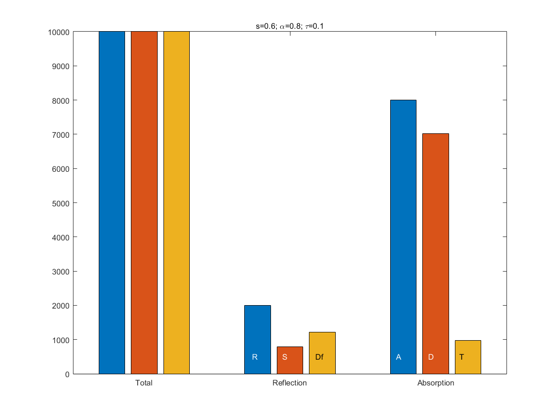
The figure Verification of the procedure for modelling absorption (dissipation and transmission) and reflection (specular and diffuse) phenomena illustrates the result of the reflection procedure (reflection=specular/diffuse, absorption=loss/transmission) in random mode, with the following acoustic parameters: scattering coefficient $s=0.6$, absorption coefficient $\alpha=0.8$, transmission coefficient $\tau=10^{-R/10}=0.1$ (attenuation index $R=10$ dB). With $10000$ realizations, the different phenomena are found (in terms of number of realizations) with the same proportions as the imposed acoustic parameters.

Verification of the procedure for modelling absorption, transmission and reflection.

Verification of the procedure for modelling absorption (dissipation and transmission) and reflection (specular and diffuse) phenomena¶

In the previous figure, only the random drawing process is modelled (note that this simulation was realized with a very simplementation of the method, not the the one implemented in the SPPS code, this last one being more performant).

The first group “Total” corresponds to the sum of the number of achievements (initial number of particles, reflection + absorption, specular + diffus + dissipation + transmission); these three quantities therefore have the exactly same value, which the initial number of sound particles (i.e. 10000).
The second group corresponds to the “Reflection” process, divided into the total number of reflections (R, 2005 particles, i.e an equivalent reflection coefficient of 0.2005, which is quite the same that the initial condition of the random process $R=1-\alpha=0.2$), specular reflections (S, 788 particles) and diffusion (Df, 1217 particles, , i.e an equivalent scattering coefficient of 1217/2005=0.61, which is quite the same that the initial condition of the random process $s=0.6$)).
The third group corresponds to the “Absorption” process, divided into the total number of absorption (A, 7995 particles, , i.e an equivalent absorption coefficient of 0.7995, which is quite the same that the initial condition of the random process $\alpha=0.8$)), dissipation (D, 7014 particles) and transmission (T, 981 particles, , i.e an equivalent transmission coefficient of 0.0981, which is quite the same that the initial condition of the random process $\tau=0.1$)).

Calculation of sound levels at observation points¶

In the SPPS code, two types of receivers are considered:

“Volume” receivers model the so-called « classical » point receivers. Since the notion of point receiver is not applicable in the SPPS code, since in theory the probability that a sound particle will pass through a point receiver is zero, it is necessary to give a volume to the receiver point, to count the number of particles that have passed through it, and thus deduce the energy density at the observation point. For a point receiver, the SPPS code returns the sound pressure level, at each time step of the calculation and for each frequency band considered;
“Surface” receivers are surface elements (like a face element of the 3D scene) on which incident sound intensities are calculated, which then makes it possible to construct acoustic maps. For a surface receiver, the code SPPS returns the sound intensity, at each time step of the calculation and for each frequency band considered.

In addition, the calculation code also determines the overall sound pressure level in the 3D model, summing the contributions of each particle, at each time step and for each frequency band.

Calculation of the sound pressure level at a volume receiver¶

The amount of energy $E_\text{rec}^{j}(n)$ (in J or W.s) in the frequency band $j$ received at a volume receiver, at the time step $n$ (i.e. to time $n \Delta t$) is equal to the sum of the energies $\varepsilon_i^{j}$ brought by each particle $i$ in the frequency band $j$, crossing the receiver volume during the time step $n$ (figure[principle_receiver_volumique]):

\[E_\text{rec}^{j}(n)=\sum_i^{N_0} \varepsilon_i^{j} = \sum_i^{N_0} \frac{W}{N} \epsilon_i^{j} \times \Delta t_i,\]

where ${N_0}$ is the total number of particles passing through the receiver volume and $\Delta t_i$ is the presence time of the particle $i$ in the receiver volume ($\Delta t_i<\Delta t$), and $\epsilon_i^{j}$ the weighting coefficient (between 0 and 1) associated with the particle $i$ in the frequency band $j$. If the calculation mode is « random », the coefficient $\epsilon_i^{j}$ is constant and equal to the unit (1). If the calculation mode is « energetic », the coefficient $\epsilon_i^{j}$ translates the cumulative loss of energy in the frequency band $j$ of the particle $i$ throughout its path due to the physical phenomena encountered (absorption by walls and obstructions, atmospheric absorption, sound transmission…). The presence time $\Delta t_i$ can also be expressed as a function of the length of the path of the particle $i$ in the receiving volume, i.e. $\ell_i$, such as $\Delta t_i=\ell_i/c$, $c$ being the velocity of the particle at the observation point. Considering a « volume » receiver is defined by a spherical volume of radius $r_\text{rec}$ (and volume $V_\text{rec}$), the energy density $w_\text{rec}^{j}(n)$ (J/m$^3$) in the volume receiver, for the frequency band $j$, is given by:

(14)¶\[\label{densite_energie_recepteur_volumique} w_\text{rec}^{j}(n)=\frac{E_\text{rec}(n)}{V_\text{rec}}= \frac{W}{N} \frac{1}{V_\text{rec}} \sum_i^{N_0} \epsilon_i^{j} \frac{\ell_i}{c}.\]

Note

The definition of the receiver volume is a crucial element for the quality and representativeness of the results. It must be large enough to count sound particles as they propagate, but not too large to make the energy density calculated at the observation point representative.

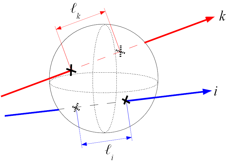
Principle of the calculation of the sound pressure level for a volume receiver¶

The energy density in the volume receiver is calculated by summing the energy contributions of each particle passing through the receiver. The contribution of the particle $i$ is calculated from the path $\ell_i$ of the particle in the volume receiver (14).

The sound intensity $I_\text{rec}^{j}(n)$ (in W/m$^2$) at the receiving point is given by:

\[I_\text{rec}^{j}(n)=c \times w^{j}_\text{rec}(n)= \frac{W}{N} \frac{1}{V_\text{rec}} \sum_i^{N_0} \epsilon_i^{j}\ell_i.\]

The sound intensity level $L_\text{I,rec}^{j}(n)$ and the sound pressure level $SPL_\text{rec}(n)$ (in dB) can then be derived from the sound intensity by the following relationships:

\[\label{LI_recepteur_volumique} L_\text{I,rec}^{j}(n)=10\log\left(\frac{P2_\text{rec}^{j}(n)}{\rho_0 c I_0}\right),\]

and

\[\label{SPL_recepteur_volumique} SPL_\text{rec}^{j}(n)=10\log\left( \frac{P2_\text{rec}^{j}(n)}{p_0^2}\right),\]

where $I_0=10^{-12}$ W/m $^2$ and $p_0=20 \times 10^{-6}$ Pa denote the reference sound intensity and sound pressure. Each of the previous quantities (energy, energy density, intensity and sound levels) are calculated for each frequency band.

Intensity vector at a volume receiver¶

The vector sound intensity $\mathbf{I}_\text{rec}^{j}(n)$ (in W/m $^2$ or J/m $^2$.s) at the receiving point, for the frequency band $j$, is defined as the sum of the energy densities carried by the velocity vector $\mathbf{v}_i$ of the particles (standard $c_i$) passing through the receiving volume:

Calculation of the lateral sound pressure level at a volume receiver¶

For the calculation of certain acoustic parameters, such as those based on lateral energy (LF with a weighting in $|\cos\theta|$ and LFC with a weighting in $\cos^2\theta$), it is necessary to consider a weighting of the sound intensity as a function of the angle $\theta$ between the observation direction of the point receiver (in principle oriented towards the sound source) and the incident direction of the particles at the receiver. As a result, the SPPS code also returns the following two quantities, homogeneous to the square of the sound pressure (i.e. in Pa$^2$):

\[\begin{split}\begin{aligned} P2_{\text{rec},\cos\theta}^{j}(n)&= \rho_0 c^2 \times w^{j}_{\text{rec},\cos\theta}(n)\\ &= \rho_0 c \frac{W}{N} \frac{1}{V_\text{rec}} \times \sum_i^{N_0} \epsilon_i^{j}\ell_i|\cos\theta_i|, \end{aligned}\end{split}\]

and

\[\begin{split}\begin{aligned} P2_{\text{rec},\cos^2\theta}^{j}(n)&= \rho_0 c^2 \times w^{j}_{\text{rec},\cos^2\theta}\\ &= \rho_0 c \frac{W}{N} \frac{1}{V_\text{rec}} \times \sum_i^{N_0} \epsilon_i^{j}\ell_i\cos^2\theta_i. \end{aligned}\end{split}\]

where $\theta_i$ is the corresponding angle for the particle $i$.

Calculation of the sound intensity level on a surface receiver¶

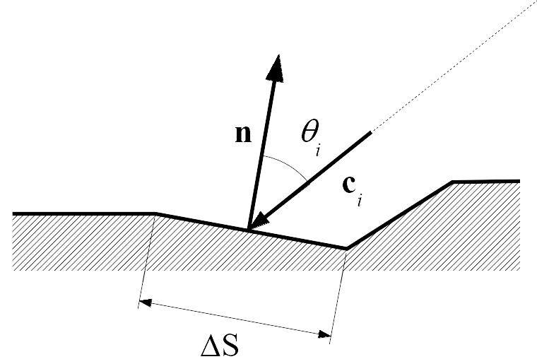
The power $W_\text{surf}^{j}$ (in W) received by a surface element of size $\Delta S$ of normal $\mathbf{n}$ is equal to the sum of the energy provided by each particle $i$ in the frequency band $j$ per time unit $\Delta t$, at the time step $n$ (i.e. at time $n\Delta t$), either:

\[W_\text{surf}^{j}(n)=\sum_i^{N_0} \frac{\varepsilon_i^{j}}{\Delta t} \frac{\mathbf{v_i}}{c}\cdot \mathbf{n}=\frac{W}{N} \sum_i^{N_0} \epsilon_i\cos\theta_i,\]

where $\mathbf{v_i}$ refers to the velocity vector (of norm $c$) of the particle $i$, $\theta_i$ the angle between normal $\mathbf{n}$ of the surface and the direction of the particle, and where ${N_0}$ is the total number of sound particles colliding with the surface element $\Delta S$.

The sound intensity $I_\text{surf}^{j}(n)$ (in W/m $^2$) received by the surface element $\Delta S$ at the time step $n$ is equal to the power received divided by the surface, either:

\[I_\text{surf}^{j}(n)=\frac{W}{N} \frac{1}{\Delta S}\sum_i^{N_0} \epsilon_i^{j} \cos\theta_i.\]

The sound level $L_\text{surf}^{j}(n)$ (in dB) can then be calculated by the following relationship:

\[\label{L_receiver_surface} L_\text{surf}^{j}(n)= 10\log\frac{I_\text{surf}^{j}(n)}{I_0},\]

where $I_0=10^{-12}$ W/m $^2$ is the reference intensity.

Principle of the calculation of the sound intensity level for a surface receiver¶

Calculation of the sound pressure level on a surface receiver¶

Equivalent to the calculation of the sound intensity level on a surface receiver, the quadratic sound pressure $P2_\text{surf}^{j}(n)$ (in Pa) received by the surface element $\Delta S$ at the time step $n$ is equal to the product of the sound intensity (without weighting the angle of incidence on the surface) by the characteristic impedance of the air $\rho_0$ that is:

\[P2_\text{surf}^{j}(n)=\rho_0\rho_0\, c \frac{W}{N} \frac{1}{\Delta S}\sum_i^{N_0} \epsilon_i^{j}.\]

The sound pressure level $L_\text{SPL,surf}^{j}(n)$ (in dB) can then be calculated by the following relationship:

\[\label{SPL_receiver_surface} L_\text{SPL,surf}^{j}(n)= 10\log\frac{P2_\text{surf}^{j}(n)}{p_0^2},\]

where $p_0=20\times 10^{-6}$ Pa is the reference sound pressure.

Avertissement

Note that the calculation of a sound pressure level for a surface is quite ambiguous. It should not be comparable to grid of punctual receivers on a plane.

Calculation of the overall sound pressure level in the model¶

The overall sound intensity $I_\text{global}^{j}(n)$ in the model, for the frequency band $j$, is calculated by summing the intensities carried by all the sound particles present $N_n$ in the model at the time step $n$ (i.e. at time $n\delta t$):

\[I_\text{global}^{j}(n)= \frac{W}{N} \frac{1}{V_\text{rec}} \sum_i^{N_n} \epsilon_i^{j}\ell_i.\]

The sound pressure level $SPL_\text{global}^{j}(n)$ (in dB) can then be calculated by the following relationship:

\[\label{SPL_global} SPL_\text{global}^{j}(n)=10\log\left( \frac{P2_\text{global}^{j}(n)}{p_0^2}\right),\]

where $p_0=20\times 10^{-6}$ Pa is the reference sound pressure.